
Fine-Tuning LLMs: Hyperparameter Best Practices
Practical hyperparameter rules for LLM fine-tuning: learning-rate warmup-stable-decay, batch-size and gradient strategies, epochs, and automated tuning workflows.

Fine-tuning large language models (LLMs) can transform general-purpose models into task-specific experts, but success hinges on optimizing key hyperparameters. Here's what you need to know:
- Learning Rate: Start with 2e-4 for LoRA fine-tuning and use a warmup-stable-decay schedule to balance speed and stability.
- Batch Size: Use the largest batch size your GPU can handle (16 or 32 recommended). Gradient accumulation is a workaround for memory limitations but doesn't speed up training.
- Epochs: 3–5 epochs are usually sufficient. Use early stopping to prevent overfitting and save compute resources.
Challenges like overfitting, catastrophic forgetting, and resource constraints make structured workflows essential. Start with smaller models and datasets to test configurations quickly, then scale up. Automated methods like Bayesian optimization or Population-Based Training (PBT) can streamline hyperparameter tuning for complex setups.
The key is balancing efficiency and accuracy - focus on quality data, monitor metrics, and refine settings iteratively to achieve optimal performance.
Key Hyperparameters to Optimize
When fine-tuning a model, three hyperparameters stand out as the most influential: learning rate, batch size, and number of epochs. These parameters directly affect how quickly the model learns, how stable the training process is, and how well the model generalizes to new data. Getting them wrong can waste resources; getting them right can lead to a model ready for deployment.
Learning Rate and Scheduling
The learning rate controls how much the model's weights adjust during each training step. Think of it as the size of the steps the model takes toward finding the best solution. A high learning rate speeds up training but risks overshooting the target or making the process unstable. On the other hand, a low learning rate ensures stability but can slow progress or leave the model stuck in less optimal solutions.
Dynamic scheduling helps manage the learning rate in three phases: warmup, stable, and decay. The warmup phase begins with a small learning rate to avoid unstable updates early on. During the stable phase, the rate remains high for efficient learning. Finally, the decay phase gradually lowers the rate, allowing the model to settle into a better solution. For LoRA fine-tuning, it's recommended to start with a learning rate of 2e-4 and use a Warmup-Stable-Decay schedule, keeping the high rate for 80% of training before sharply reducing it by 10%. As Yiren Lu, Solutions Engineer at Modal, puts it:
"The bigger the learning rate, the faster fine-tuning goes, but you have to balance that against the risk of overshooting the optimal solution or causing unstable training."
Keep an eye on your training loss. Sudden spikes or "NaN" (Not a Number) values are red flags - if you see them, lower your learning rate immediately. A good rule of thumb is to set warmup steps to 10% of the total training steps.
Next, let’s look at how batch size can further impact training efficiency and stability.
Batch Size and Gradient Accumulation
Batch size determines how many training examples are processed before the model updates its weights. Larger batch sizes provide more stable gradient estimates, but they require more GPU memory. To maximize efficiency, aim to use the largest batch size your GPU can handle.
If memory constraints limit your batch size, gradient accumulation can help. This technique processes several smaller batches, accumulating their gradients before updating the model's weights. For LoRA fine-tuning, an effective batch size is typically 16 or 32.
However, gradient accumulation has its limits. It doesn’t increase training speed; instead, it’s a workaround for memory issues. As Google Research notes:
"Gradient accumulation simulates a larger batch size than the hardware can support and therefore does not provide any throughput benefits. It should generally be avoided in applied work."
Use gradient accumulation only if your batch size is extremely small (e.g., 1 or 2) to maintain training stability. If your GPU can handle a batch size of 16 or more, gradient accumulation won’t provide any additional benefits and may complicate hyperparameter tuning. Also, remember that adjusting the batch size often requires re-tuning the learning rate, as the two are closely linked. Tools like Hugging Face's auto_find_batch_size can help identify the largest feasible batch size for your hardware.
Now, let’s turn to the final piece of the puzzle: determining the right number of epochs.
Number of Epochs and Early Stopping
An epoch is a single pass through the entire training dataset. The challenge lies in finding the balance between underfitting (not learning enough) and overfitting (memorizing the training data instead of understanding broader patterns).
For most fine-tuning tasks, 3–5 epochs are sufficient. Monitor the validation loss closely and use early stopping to avoid overfitting and save compute resources. As Armin Norouzi from Lakera AI explains:
"Implementing early stopping mechanisms is crucial to prevent overfitting. If the model's performance plateaus or degrades on the validation set, training can be halted to avoid further overfitting."
Early stopping works well with checkpointing, which saves the model's best state before overfitting begins. This becomes especially important with smaller datasets, as they are more susceptible to overfitting.
Optimization Techniques for Fine-Tuning
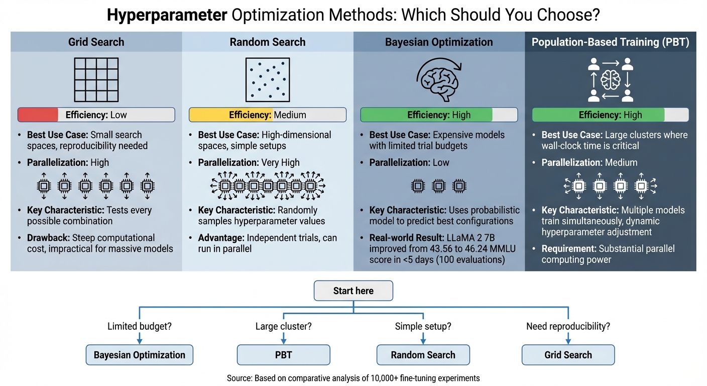
LLM Fine-Tuning Hyperparameter Optimization Methods Comparison
Once you've decided on the key hyperparameters, the next challenge is figuring out how to fine-tune them effectively. Automated optimization methods can simplify this process by systematically exploring different configurations.
Grid Search and Random Search
If you're just starting out, it's worth trying simpler methods like grid search or random search before diving into more advanced techniques.
Grid search involves testing every possible combination of hyperparameters. While this guarantees a thorough exploration of the search space, the downside is its steep computational cost. The more parameters you add, the more the cost skyrockets - making grid search less practical for massive models like LLMs with billions of parameters.
Random search, by contrast, randomly samples hyperparameter values from predefined distributions. This approach can be surprisingly effective because only a handful of hyperparameters tend to have a major impact on performance. Plus, since each trial is independent, you can run multiple experiments in parallel. For high-dimensional spaces, this makes random search a practical and efficient starting point.
Bayesian Optimization
Bayesian optimization takes a smarter approach by treating hyperparameter tuning as a problem to be learned. It uses a probabilistic model (often Gaussian Processes) to predict which hyperparameter sets are most likely to perform well based on prior results. This method balances exploring new possibilities and focusing on promising configurations.
This is particularly useful for expensive training setups. Take, for instance, a January 2024 project by researchers from Polytechnique Montréal and Huawei-Canada. They fine-tuned a LLaMA 2 7B model using LoRA on 67,000 instructions. Using Bayesian optimization (via the TPE algorithm in NNI), they completed 100 evaluations across four NVIDIA A100 80GB GPUs. The result? An optimized model with an average MMLU score of 46.24, a notable improvement over the baseline score of 43.56 - all achieved in under five days. Since Bayesian optimization typically requires fewer trials than random search, it’s an excellent choice for large-scale models where training runs are resource-intensive.
Population-Based Training (PBT)
If you're working with abundant computing resources, Population-Based Training (PBT) offers a compelling alternative. Unlike Bayesian methods, which focus on reducing the number of evaluations, PBT emphasizes minimizing wall-clock time by leveraging parallelism.
With PBT, multiple models train simultaneously, forming a "population." Periodically, weaker models are replaced by stronger ones, and hyperparameters are adjusted dynamically to maintain diversity. This continuous adaptation during training - rather than fixing hyperparameters at the start - can save significant time by building on partially trained models.
The main tradeoff? PBT demands substantial parallel computing power. It's most effective for projects where reducing total training time is a priority, and a robust GPU budget is available.
| Method | Efficiency | Best Use Case | Parallelization |
|---|---|---|---|
| Grid Search | Low | Small search spaces, reproducibility needed | High |
| Random Search | Medium | High-dimensional spaces, simple setups | Very High |
| Bayesian Optimization | High | Expensive models with limited trial budgets | Low |
| PBT | High | Large clusters where wall-clock time is critical | Medium |
Best Practices for Hyperparameter Workflows
Structured workflows are the backbone of effective hyperparameter tuning. They ensure each training iteration moves the needle on model performance while balancing speed, cost, and accuracy. The difference between mediocre and expert-level results often lies in the approach.
Start with Smaller Models and Datasets
Kick things off with a smaller model and a subset of your dataset. For example, instead of diving straight into a 70B parameter model, begin with an 8B model. This strategy drastically cuts down experiment time, allowing you to test various hyperparameter configurations without depleting your compute budget.
"Choosing an initial configuration that is fast and minimizes resource use will make hyperparameter tuning much more efficient." - Google Research, Tuning Playbook
Research shows that experimenting with smaller models like Llama-3-8B or Mistral-7B can yield excellent insights. Once you’ve identified hyperparameter settings that work well on a smaller scale, you can scale up to the full model and dataset with confidence. This step-by-step approach also helps catch issues like overfitting early, when they’re cheaper to address. In fact, starting with as few as 50 high-quality training examples can be enough to gauge whether your model is hitting accuracy goals before committing to larger datasets.
Once you’ve nailed down stable settings in these smaller experiments, the focus shifts to monitoring metrics for further refinement.
Monitor Metrics and Prevent Overfitting
Keeping an eye on the gap between training loss and validation loss is critical for spotting overfitting. If training loss keeps dropping but validation loss starts climbing, it’s a clear sign your model is memorizing the training data rather than learning patterns that generalize. Regularly track metrics and use early stopping when validation performance stops improving or begins to degrade.
In addition to loss, monitor task-specific metrics like accuracy, F1 score, or BLEU to ensure your model is performing well in a functional context. Checkpoint frequently to capture the best-performing model state instead of relying solely on the final epoch’s output. This is especially crucial for large language models (LLMs), which are prone to overfitting, particularly when fine-tuned on smaller, domain-specific datasets.
With early stopping in place, you can further stabilize training by incorporating gradient clipping.
Use Gradient Clipping
Gradient clipping is a must for keeping training stable, especially when working with large models or experimenting with higher learning rates. Without it, you risk exploding gradients, where weight updates become excessively large and cause the training process to spiral out of control.
"Watch for validation metrics diverging from training metrics... If loss spikes or becomes NaN, reduce learning rate." - Predibase
This technique is particularly useful when pushing learning rates to accelerate convergence. By capping gradients, you can experiment with aggressive hyperparameters without destabilizing training. For LoRA fine-tuning, combining gradient clipping with a starting learning rate of around 2e-4 provides a solid baseline that can be adjusted based on how training progresses.
Using Latitude for Hyperparameter Fine-Tuning

Hyperparameter tuning is all about creating a workflow that gathers insights, incorporates feedback, and leads to better performance. Latitude's open-source platform simplifies this process, helping teams observe model behavior and adjust configurations based on real-world data.
By building on the strategies mentioned earlier, Latitude makes the entire tuning process more efficient.
Observability and Evaluation Tracking
To make informed decisions and ensure reproducibility, tracking hyperparameter experiments is crucial. Latitude allows teams to log every prompt run with full context, output, and metadata, including custom details like user type or data source.
Its evaluation tracking feature supports batch evaluations, enabling comparisons of hyperparameter configurations across multiple metrics. After external fine-tuning, you can bring the model back into Latitude, set it up as a provider, and measure the results against your baseline. This closed-loop approach ensures that every adjustment is tested with real data before moving to production.
These observations seamlessly feed into the next round of tuning.
Feedback Collection for Iterative Tuning
Human feedback is a limited but invaluable resource. Latitude tackles this challenge by offering human-in-the-loop evaluation tools, allowing domain experts to review model responses and provide structured feedback. This collaborative setup bridges the gap between engineers and domain experts, enabling them to refine prompts and improve model behavior together.
"No model is perfect, and user interactions provide a goldmine of insights into its strengths and weaknesses." - Aarti Jha
Using Latitude, you can create datasets of high-quality, manually reviewed outputs that act as ground truth for optimizing hyperparameters. These datasets can be exported as CSV files to external fine-tuning pipelines, where you can test various hyperparameter configurations. Once the tuning is complete, re-import the model into Latitude and validate its performance against the original curated datasets. Features like version control and tagging help track changes and roll back if needed.
This continuous feedback loop drives ongoing improvements in the model.
Continuous Improvement Pipelines
Hyperparameter optimization isn’t a one-and-done task - it’s an ongoing process. Latitude supports this iterative cycle by enabling a "flywheel" approach: evaluate, collect feedback, tweak hyperparameters, and measure the results. Automated logging captures every experiment, making it easy to compare configurations and identify what truly works.
"Optimizing model output requires a combination of evals, prompt engineering, and fine-tuning, creating a flywheel of feedback that leads to better prompts and better training data." - OpenAI
With Latitude, this cycle becomes a streamlined process, ensuring consistent improvements over time.
Conclusion
Hyperparameter optimization is the backbone of fine-tuning large language models (LLMs). According to Google Research, even with advancements, deep neural networks still involve a fair amount of effort and guesswork. To streamline the process, start with default settings (like a 2e-4 learning rate for LoRA) and tweak one parameter at a time.
Why does this matter? Because using incorrect hyperparameters can lead to model divergence or waste precious GPU hours. Large-scale studies, involving over 10,000 fine-tuning experiments, reveal that testing a few carefully chosen configurations often yields results comparable to exhaustive grid searches. In other words, efficiency is just as crucial as accuracy.
Optimization is an ongoing process. Tools like Latitude simplify this journey by offering features like observability, evaluation metrics, and feedback collection. These platforms bring structure to what was once trial-and-error, turning it into a scalable, scientific method.
Focus on quality data, start with smaller experiments, and build a repeatable system that improves with each iteration. With well-tuned hyperparameters and a structured workflow, your models are set to perform consistently in production.
FAQs
What is the ideal starting learning rate for LoRA fine-tuning, and why is it important?
For LoRA fine-tuning, it's best to begin with a low learning rate, usually around 1e-4 or less. This approach helps keep the training process stable and lets the model adjust to new tasks without veering off course or overfitting.
Using a cautious learning rate ensures that fine-tuning makes gradual adjustments. This way, the model retains its pre-trained knowledge while adapting to specific tasks. On the other hand, starting with a higher learning rate can make the process unstable and produce less-than-ideal results - especially when dealing with large language models (LLMs).
What’s the best way to manage batch size while considering memory limitations during LLM fine-tuning?
Managing batch size while working within memory limits is all about finding the right balance between performance and available resources. A good starting point is to use a smaller batch size to ensure your system can handle the workload without running into memory issues. From there, you can slowly increase the batch size if your hardware allows, keeping a close eye on memory usage to prevent crashes or performance slowdowns.
If memory remains a limitation, you can explore methods like gradient accumulation. This technique allows you to mimic larger batch sizes by breaking the workload into smaller, more manageable batches. It’s an effective way to boost performance while staying within the boundaries of your hardware's capabilities.
What makes early stopping important for preventing overfitting during LLM fine-tuning?
Early stopping plays a key role in machine learning by halting training before a model starts overfitting - essentially preventing it from memorizing the training data. This helps the model retain its ability to generalize well to new, unseen data, which is crucial for dependable performance in practical scenarios.
By keeping an eye on metrics like validation loss, early stopping helps pinpoint the ideal moment to stop training. This technique strikes a balance between achieving effective results and minimizing training time, all while cutting down on unnecessary computational expenses.
